Creating Functional Mock-up Unit (FMU) models using C++

In our previous blog post "The history of system simulations", we introduced the Functional Mock-up Unit (FMU) – a standard container format for exchanging dynamic models between simulation tools. The behaviour of FMUs can be modelled from data using machine learning (ML) techniques and/or using first principles of physics. ML techniques can allow to create models without needing to understand fundamental equations or needing to do a thorough analysis of the system that is being modelled, if sufficient data can be available. On the other hand, explicit modelling using first principles of physics can often yield more accurate simulations and help in our understanding of the target system’s behaviour. In this blog post, we describe how to create an FMU based on first principles by using C++, which gives modellers full control over capturing both the model’s behaviour and its internal states. We illustrate this using a simple robot arm model with two degrees of freedom.

Background

At DNV, many experts are working on projects that involve simulations. The Open Simulation Platform (OSP) initiative produced various developer and end-user tools that use the Functional Mock-up Interface (FMI) standard. Today, FMI is a de-facto standard for many modelling tools that export simulation models. The FMI standard defines, amongst many other aspects, the following specifications that facilitate re-using models in different simulation environments:

Standard interface – allows external tools to interact with models for simulation.
Metadata – provides information on available input and output ports, parameters and their data types. In addition, model-vendor-specific information can be included in this metadata.
File container – defines the layout of the exported models, metadata and documentation, organized in a single file archive (with .fmu extension), called the Functional Mock-up Unit (FMU).
Calling sequence – defines a model’s lifecycle during simulation, i.e. initialization, stepping and teardown.

Although modellers can create FMUs from scratch, this process is often tedious and prone to mistakes, especially when they are modelling in plain C++. To simplify this task, OSP offers a C++ framework called cpp-fmus, which allows for more explicit modelling and supports the automated creation of FMUs.

Overview of cpp-fmus

cpp-fmus is a framework that enables model behaviour to be defined by extending a C++ base class. To use it, modellers implement a set of interface functions specified by this base class, which are invoked during simulation in accordance to the FMI specification. These functions are called at various stages fo the simulation lifecycle – for example, when reading or outputting data, once at initialization and termination, and when solving equations.

cpp-fmus/
├── cmake/
├── cppfmu/
├── fmi/
├── src/
│   ├── model1/
│   │   ├── sources/
│   │   │   └── fmu.cpp
│   │   └── modelDescription.xml
│   └── model2/
├── tools/
└── CMakeLists.txt

Figure 1. cpp-fmus project layout

The framework expects modellers to organize their files in a specific layout, as shown in Figure 1. Each model has its down directory (e.g. model1 and model2) under the main src directory, containing the source code (fmu.cpp) and metadata (modelDescription.xml). Additional directories such as cmake, cppfmu, fmi and tools support the cpp-fmus framework in generating FMUs from the contents of the src directory. The cppfmu folder includes a submodule that provides a set of interfaces and helper functions to help simplifying the development of FMI-compliant C++ code.

As a minimum for creating an FMU, two files are required: 1) the model description file (modelDescription.xml) and 2) the fmu source file (fmu.cpp). The model description file serves as a metadata for the FMU, containing essential information about the model and its source files. It also defines how the modeller has implemented the FMU interface. In the following sections, we will explain how these files are created using the 2 DoF robot arm model example.

Two Degrees of Freedom (DOF) Robot Arm Model

Models of a multi-DoF robot arm are extensively discussed in various books and articles. In this blog post, we are considering a robot arm with two links with length $l_1$ and $l_2$ as shown in Figure 2. Normally, finding a dynamic model of the robot arm involves deriving equations of kinetic and potential energies using Lagrangian mechanics [1]. The final equation including the PID control is shown in Equation \ref{eq:dynamic}. For the details of deriving this equation, readers are referred to [1].

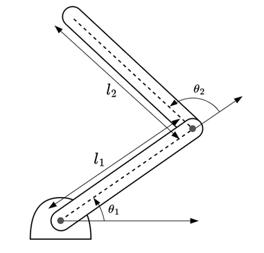
Figure 2: Two degress-of-freedom robot arm

$$ \ddot{q} = \begin{bmatrix} \ddot{\theta}_1 \\ \ddot{\theta}_2 \end{bmatrix} = \underbrace{B(q)^{-1} \left[ -C(\dot{q}, q) - g(q) \right]}_{\text{dynamic}} + \underbrace{ \begin{bmatrix} K_{P1}(\theta_{1r} - \theta_1) + K_{D1}\dot{\theta}_1 + K_{I1}e_1 \\ K_{P2}(\theta_{2r} - \theta_2) + K_{D2}\dot{\theta}_2 + K_{I2}e_2 \end{bmatrix} }_{\text{PID control}}\tag{1}\label{eq:dynamic} $$

Equation \ref{eq:dynamic} consists of two parts, first describing inertial, Coriolis and centrifugal forces, denoted by matrices $B$ and $C$, and gravitational term $g$. The second part models the PID control action, which aims to minimize the difference between the target set points in radians ($\theta_{1r}$ and $\theta_{2r}$) and the current position of the robot arm ($\theta_1$ and $\theta_2$). Computing the position of each link for the next simulation step $t_{n+1}$ requires calculating the torque $\ddot{\theta}$ at each link's joint using Equation \ref{eq:dynamic} and deriving new values for $\dot{\theta}$ and $\theta$. The position of the end effector (the tip of the second link) can then be found using forward kinematics.

C++ Implementation of the 2-DoF Robot Arm

The dynamics of the 2-DoF robot arm are implemented in C++ and exported to FMU using cpp-fmus. The first step is to define the layout of the FMU model’s input and output ports and the parameters in the modelDescription.xml file, as shown in Figure 3.

<?xml version="1.0" encoding="utf-8" ?>
<fmiModelDescription
    fmiVersion="2.0"
    modelName="manipulator"
    guid="@FMU_UUID@"
    description="Two degrees freedom Robot Arm"
    author="DNV"
    version="0.1">

    <CoSimulation
        modelIdentifier="manipulator"
        canHandleVariableCommunicationStepSize="true" />

    <ModelVariables>
        <ScalarVariable name="l1" valueReference="0" causality="parameter"  variability="fixed"><Real start="1.0"/></ScalarVariable>
        <ScalarVariable name="l2" valueReference="1" causality="parameter"  variability="fixed"><Real start="1.0"/></ScalarVariable>
        <ScalarVariable name="m1" valueReference="2" causality="parameter"  variability="fixed"><Real start="0.5"/></ScalarVariable>
        <ScalarVariable name="m2" valueReference="3" causality="parameter"  variability="fixed"><Real start="0.5"/></ScalarVariable>

        <ScalarVariable name="q1"   valueReference="4"   causality="output" variability="continuous"><Real/></ScalarVariable>
        <ScalarVariable name="q2"   valueReference="5"   causality="output" variability="continuous"><Real/></ScalarVariable>
        <ScalarVariable name="ref1" valueReference="6"   causality="input" variability="continuous"><Real start="0.0"/></ScalarVariable>
        <ScalarVariable name="ref2" valueReference="7"   causality="input" variability="continuous"><Real start="0.0"/></ScalarVariable>

        <ScalarVariable name="Kp1" valueReference="8"  causality="parameter"   variability="fixed"><Real  start="300.0"/></ScalarVariable>
        <ScalarVariable name="Kd1" valueReference="9"  causality="parameter"   variability="fixed"><Real  start="50.0"/></ScalarVariable>
        <ScalarVariable name="Ki1" valueReference="10" causality="parameter"  variability="fixed"><Real  start="1.0"/></ScalarVariable>
        <ScalarVariable name="Kp2" valueReference="11"  causality="parameter"   variability="fixed"><Real  start="300.0"/></ScalarVariable>
        <ScalarVariable name="Kd2" valueReference="12"  causality="parameter"   variability="fixed"><Real  start="50.0"/></ScalarVariable>
        <ScalarVariable name="Ki2" valueReference="13" causality="parameter"  variability="fixed"><Real  start="1.0"/></ScalarVariable>
    </ModelVariables>

    <ModelStructure>
        <Outputs>
            <Unknown index="4" />
            <Unknown index="5" />
        </Outputs>
    </ModelStructure>

</fmiModelDescription>

Figure 3. The modelDescription.xml file of the 2 DoF robot arm

This file contains a list of static model parameters—such as the lengths ($l_1$, $l_2$) and masses ($m_1$, $m_2$) of the links, and the proportional ($K_{P1}$, $K_{P2}$), integral ($K_{I1}$, $K_{I2}$), and derivative ($K_{D2}$, $K_{D2}$) gains for the PID controller. These parameters are marked with variability="fixed" and have a causality type of "parameter", indicating that their values remain constant throughout the simulation.

The model also defines two inputs, ${ref}_1$ and ${ref}_2$, which represent the desired joint angle setpoints, and two outputs, $q_1$ and $q_2$, which correspond to the current joint angles of the robot arm links, which are shown as $\theta_1$ and $\theta_2$ in Figure 2. Each variable in the FMU is assigned a unique "valueReference" ID, which allows its value to be accessed programically via modelDescription.xml. In this example, the IDs range from 0 to 13.

Once the model interface is defined in modelDescription.xml, it is time to implement the model’s behaviour in the fmu.cpp file.

To avoid cluttering the figure with implementation details, we only show the overall structure of the model, as shown in Figure 4 (left). The source code for this example is available on GitHub at dnv-opensource.

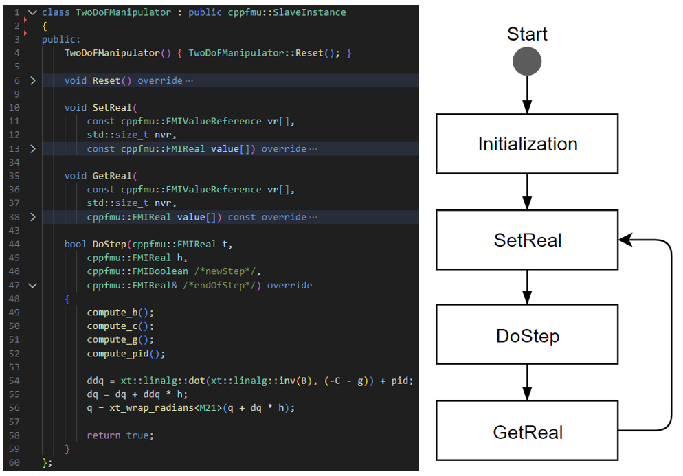
Figure 4: Implementing the dynamics of the 2 DoF robot arm (left) and the execution flow of cpp-fmus (right)

The main class file that extends cpp-fmus’ SlaveInstance is called TwoDoFManipulator and implements three interface methods called SetReal, GetReal and DoStep. In the SetReal method, the model reads the joint angle reference value written by the external environment (e.g. a user), which will be used to drive the robot arm to a specific position. The GetReal method is used to output values computed by the model (i.e. current joint angles). The method’s input arguments vr, nvr, and value correspond to value references, the number of value references, and values of the input and output ports for the current simulation step, respectively.

The main dynamics of the robot arm is implemented in the DoStep function, where the matrices for B, C and g and the output of the PID controller are computed, as shown in lines 49-56 in Figure 4. The angular velocities and positions of the joints are computed using a simple numerical method.

The cpp-fmus framework calls the prescribed functions in sequence during simulation. The right-hand side of Figure 4 shows a simplified overview of the execution flow when this code is exported and simulated as an FMU.

Creating an FMU

The cpp-fmus framework includes a CMakefile.txt file that automates the process of generating an FMU from the source code and model modelDescription.txt file described in the previous section. To build an FMU, users can execute the following commands from the root directory of the cpp-fmu tool:

git submodule init
git submodule update
cmake build
cd build
cmake .. # Append “-DCMAKE_BUILD_TYPE=Release” for Linux build
cmake --build . --config Release --target <model_directory_name>_fmu # Remove “–config Release” for Linux Build

Note that the commands listed above are used for cases where the FMU does not depend on third-party libraries. Users may need to perform additional steps to import third-party libraries. For example, in our use case, the FMU depends on the xtensor and openblas libraries. In the provided example, these are installed using the conan C++ package manager (https://conan.io/). To ease the build process, we created a build script called buildfmu that automates the entire build process and generates a final FMU file for the 2DoF robot arm model.

Simulating an FMU

There are many tools available that can import and simulate an FMU. In this blog post, we used DNV’s Simulation Trust Center (https://store.veracity.com/simulation-trust-center) to generate simulation data. We validated that we could actuate the robot arm to different desired positions, for example, between $[\pi/2,-\pi/2]$ and $[-\pi/2,\pi/2]$. A screenshot of simulation data in STC and the animated movements of the robot arm from the simulation data are shown in Figures 5 and 6, respectively.

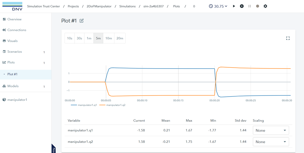
Image of simulation results for 2 DoF robot arm in STC. — Figure 5: Simulating 2 DoF robot arm in Simulation Trust Center (STC)

Gif of simple visualization of a 2 DoF robot arm moving. — Figure 6: Moving a robot arm to different joint angle targets

Alternative FMU Generation Tools for C++

In this blog post, we discussed using cpp-fmus for creating FMUs based on C++ code. We would like to point out that several other tools have recently been developed to help C++ developers create FMUs. Below, we summarize some of the notable ones.

fmu4cpp (https://github.com/Ecos-platform/fmu4cpp) [MIT license] - This tool simplifies FMU creation by automatically generating the modelDescription.xml file based on variable registration in the source code. In addition, the tool manages variable reading and writing variables during simulation, so functions such as SetReal or GetReal do not need to be implemented manually.
fmiCpp (https://marine-ict.pages.sintef.no/fmicpp/core) [Big Time Public License] – This framework enables fast prototyping of dynamic simulation models in C++. It supports reusing pre-compiled modules when implementing new models. Similar to fmu4cpp, fmiCpp manages reading and writing variables on FMU’s input and output ports, eliminating the need for implementing getter and setter methods. Additionally, it offers methods to split the solver’s operations into different stages.
fmipp (https://github.com/fmipp/fmipp) [FMI++ license] – Another high-level utility that provides utilities for exporting or import FMUs.

Conclusion

This blog post illustrates the process of creating a Functional Mock-up Unit (FMU), an open standard model container designed for co-simulation, using a 2-DoF robot arm as an example. C++ is used as a primary modelling language to demonstrate explicit modelling using the first principles and interacting with low-level FMI APIs via cpp-fmus. The robot arm model together with a PID controller were simulated in DNV’s Simulation Trust Center (STC) to showcase dynamic movements of the two link’s joint according to the set points fed to the controller.

Today, co-simulation is increasingly adopted across engineering disciplines to validate and verify the behaviour of complex integrated systems by interconnecting self-contained components. Looking ahead, co-simulation is expected to play a key role in assurance processes, particularly in generating evidence through data collection. Co-simulation also helps system integrators adopt models created using different modelling paradigms due to their self-contained nature, which is largely beneficial in real-world scenarios where different model vendors may prefer different technologies in creating their models.

To support engineers as well as modelling tools in adopting FMI standards within their workflows, more controlled FMU generating tools, such as CppFmu, are highly beneficial. While data-driven modelling approaches using regression methods and advanced machine learning techniques help engineers create models without prior knowledge of the target system’s behaviour, physics-based modelling techniques still offer more detailed insights into the underlying physical processes.

For several alternative approaches to creating an FMU, see the links below!

Reference

R. M. Murray, Z. Li, and S. S. Sastry, A mathematical introduction to robotic manipulation. CRC press, 2017.