Creating Functional Mock-up Unit (FMU) models from machine learning models

Imagine that you are trying to simulate a system, e.g. a wind farm or a ship, but you do not have the simulation model of any component yet, e.g. a wind power engine or the ship’s engine. You do, however, have a lot of data of this component, measured in the field. These days, it is relatively straightforward to make a simple machine learning (ML) model of this component from data, using e.g. TensorFlow. Once you have your ML model, you want to be able to use that as a digital twin in simulation-based testing. In this blog post, we describe a new tool and approach for creating ML models for simulation-based testing.

Background

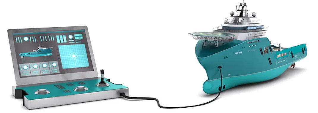
The use of simulations and digital twins has become prominent in recent years. At DNV, we have many experts working on simulation-based testing of systems, e.g. hardware-in-the-loop (HIL) or software-in-the-loop testing of systems for the assurance and certification of these systems. Examples include the HIL testing of marine control systems, such as dynamic positioning systems or power management systems. In addition, digital twin systems can be used for predictive maintenance, anomaly detection, or to verify that components are developed up to standard for system integration.

3D rendering of a ship coupled to a laptop

An example of the use of simulation-based testing for system integration comes from the Open Simulation Platform (OSP) initiative, which started as a joint industry project with several maritime industry partners. The OSP initiative developed open-source tools and working methods, primarily for co-simulation of systems. The OSP framework is built on the Functional Mockup Interface (FMI) standard, which is a free standard that defines containers and interfaces for dynamic simulation models, supported and maintained by the Modelica Association Project. The FMI standard ensures that simulation models, each packaged as a Functional Mockup Unit (FMU), and digital twin equipment easily can be interfaced and re-used across organizations. In addition, by wrapping a software component as an FMU, they can be used as black boxes, so as not to expose sensitive intellectual property (IP).

Image showing 6 people working on constructing digital twin models

Based on the OSP initiative and framework, DNV has developed the Simulation Trust Center (STC). The STC is a cloud-based platform for secure collaboration towards the simulation of complex systems. Users can securely upload their FMU models to the STC, configure how different models are connected for a system simulation via an easy-to-use graphical user interface, set up simulation configurations and scenarios, run time-series simulations, and evaluate the simulation results via graphs or downloading data into spreadsheets for further analysis and visualization. Given that users can give their collaborators limited access for only running simulations, and do not need to share the simulation models themselves, an extra layer of IP protection is added by the STC.

In previous blog posts, we explained several ways of creating simulation models. In this blog post, we focus specifically on the creation of machine learning (ML) models and making FMUs of those for your co-simulations.

Intro: From data to ML model

To provide a concrete example of how one can go from data to ML-based simulation model, we use a publicly available dataset of a wind turbine. In this section, we give an example of making a simple ML model, based on this dataset. You can skip ahead to “From ML model to FMU”, if you do not need this intro. The dataset in question is hosted on Kaggle, which also provides excellent tutorials to learn programming, Python, and introductions to machine learning and deep learning. Thus, we keep the introduction here brief.

The wind turbine dataset contains data from a field-deployed and functioning wind turbine’s scada system in Türkiye. The data files include the recorded date/time, the active power generated by the turbine for that moment, the wind speed, the theoretical power curve values that the turbine generates given the wind speed (as given by the turbine manufacturer), and the wind direction. Figure 1 provides the first rows of data (‘head’) of the wind turbine dataset. Thus, we can train a simple neural network to predict the active power production (model output), given a certain wind speed and wind direction (model input). Of course, it can also be considered if the date/time should be input data to the model as well. For simplicity, we do not include it here, but it is completely valid to consider that, and it can also be used to discover hourly, daily, or seasonal trends.

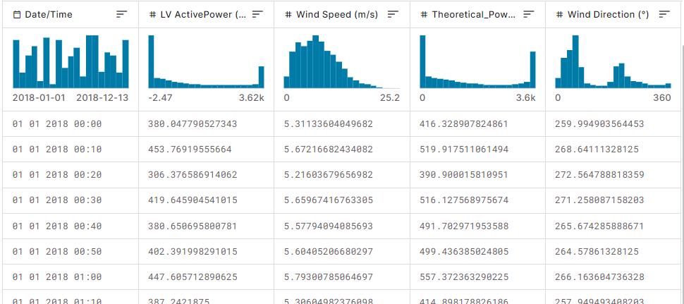
Image of the first rows of the wind turbine dataset table — Figure 1: First rows of data from the wind turbine dataset (source: kaggle.com)

Now that we have determined the input and output for the neural network (NN), we can come up with a design for the NN. Using Tensorflow and Keras (subclassing from tf.keras.Model), we create a simple design, with 2 inputs (wind speed and wind direction), 2 hidden layers that each have 32 units, and a single unit in the output layer for the power prediction:

# 2 hidden layers, 32 units each 
self.dense1 = tf.keras.layers.Dense(32, activation=tf.nn.relu) 
self.dense2 = tf.keras.layers.Dense(32, activation=tf.nn.relu) 
# output layer 
self.dense3 = tf.keras.layers.Dense(1, activation=None)

Image of a neural network with 2 inputs, 32 units in 2 hidden layers and 1 output — Figure 2: Visualization of a neural network with 2 inputs, 32 units in 2 hidden layers, and 1 output, created using NN-SVG with random weights.

We run through standard steps of data normalization and creating training and validation datasets (and test sets, if you want to test performance). We configure the model for training (optimizer RMSprop, loss “mse”), train the NN (i.e. fit for a certain number of epochs), and save it:

power_model.fit(train_power, validation_data=val_power, epochs=num_epochs_power) 
# potentially add code to check training progress, normalize the data, etc. 
# store the model: 
power_model_path = Path(Path().absolute(), "power") 
power_model_path_weights = Path(Path().absolute(), "power") 
power_model.save_weights(power_model_path_weights)
power_model.save(power_model_path)

Now that the model is trained, we can save it using ONNX, an open standard for ML interoperability, allowing us to store the ML model for usage with other frameworks:

# Load the saved keras model
keras_model = tf.keras.models.load_model(power_model_path) 
# Convert to onnx model and save as .onnx
onnx_model, _ = tf2onnx.convert.from_keras(keras_model) 
onnx_model_path = Path(Path().absolute(), "power.onnx") 
onnx.save(onnx_model, onnx_model_path)

The ONNX model can be graphically inspected with tools such as netron.app:

ONNX model displayed graphically

In the next section, we discuss how the ONNX model can be converted to an FMU.

From ML model to FMU

To use the aforementioned ML model with OSP or STC, we need to convert it to an FMU. To this end, DNV has developed the open-source, publicly available MLFMU tool. After you export your trained ML model into ONNX format, the MLFMU tool will use the ONNX file to create an FMU. To do this, you need to create an FMU interface specification .json file, which maps the FMU’s inputs, parameters and outputs to the ML model’s inputs and outputs, and you may specify whether the model uses time (see advanced usage):

{
    "name": "MyMLFMU",
    "description": "A Machine Learning based FMU",
    "usesTime": true,
    "inputs": [
        {
            "name": "input_1",
            "description": "My input signal to the model at position 0",
            "agentInputIndexes": ["0"]
        }
    ],
    "parameters": [
        {
            "name": "parameter_1",
            "description": "My input signal to the model at position 1",
            "agentInputIndexes": ["1"]
        }
    ],
    "outputs": [
        {
            "name": "prediction",
            "description": "The prediction generated by ML model",
            "agentOutputIndexes": ["0"]
        }
    ]
}

For the wind power model, the interface .json file looks like this:

{
    "name": "WindToPower",
    "description": "A Machine Learning-based FMU that outputs the estimated power output of a wind turbine, given the wind speed and direction.",
    "inputs": [
        {
            "name": "windSpeed",
            "description": "The speed of the wind",
            "agentInputIndexes": [
                "0"
            ]
        },
        {
            "name": "windDirection",
            "description": "The direction of the wind",
            "agentInputIndexes": [
                "1"
            ]
        }
    ],
    "parameters": [],
    "outputs": [
        {
            "name": "power",
            "description": "The estimated wind turbine power output",
            "agentOutputIndexes": [
                "0"
            ]
        }
    ],
    "states": []
}

Now that you have both an .onnx model file and a .json interface file, you can use the MLFMU tool to convert the model to an FMU. Say your files are called example.onnx and interface.json and they are in your current working directory, you can simply run:

mlfmu build

Alternatively, you can specify the location of these files:

mlfmu build --interface-file .\examples\wind_to_power\config\interface.json --model-file .\examples\wind_to_power\config\example.onnx

This will generate an .fmu file, which can then be used with OSP or STC.

Running the FMU on STC

Once your FMU is ready, you can upload the models in STC and create a project, where the models are loaded and connected in the model canvas, see Figure 3 and Figure 4.

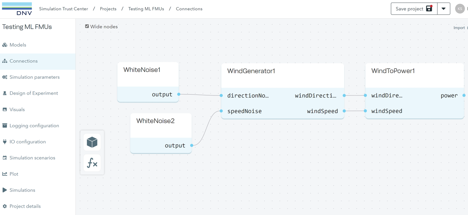
Connections View in the Simulation Trust Center, showing the imported ML FMU models — Figure 3: Connections View in STC, showing the imported ML FMU models, WindGenerator and WindToPower, and how they are connected to each other.

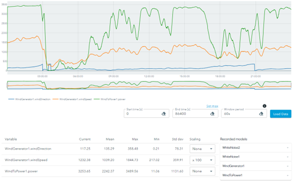
Simulation Results for the ML FMU models in the Simulation Trust Center — Figure 4: Simulation results plot in STC, showing output data from the WindGenerator and WindToPower ML FMU models.

Advanced usage: models with state

The above example contained a simple ML model that does not have state, i.e. it does not remember or carry over information from one time step to another. You may have other simulation models though where this is necessary, for example for LSTM ML models, a type of recurrent NN model. To make these kinds of models, it is necessary to add a model wrapper before converting to ONNX and using the MLFMU tool, such that you clearly define the inputs, outputs and model state for the ML model. This is described in more detail on the MLFMU tool’s GitHub pages.

Creating Functional Mock-up Unit (FMU) models from machine learning models

Table of Contents

Background

Intro: From data to ML model

From ML model to FMU

Running the FMU on STC

Advanced usage: models with state

More blog posts on Simulations and FMU models

Points of Contact